Capital Budgeting

Capital budgeting is the structured process of evaluating and ranking major long-term investments by quantifying expected cash flows, assessing risk, and comparing returns against a discount rate before committing funds. Its core methods are net present value—the preferred value-maximizing metric—internal rate of return, payback period, profitability index, and accounting rate of return.

Why major business investments require structured capital budgeting

Major business investments carry a weight that ordinary operating decisions do not. When a company commits to a new factory, a fleet of equipment, an acquisition, or a multi-year software platform, it is locking up substantial resources for years, often decades. These commitments are largely irreversible: specialized machinery has limited resale value, and capital sunk into construction cannot easily be recovered if demand shifts. Because the sums involved are large relative to annual cash flow, a single poor decision can strain liquidity, raise borrowing costs, and depress earnings for several reporting periods. Structured capital budgeting exists to impose discipline on decisions of this magnitude, forcing managers to quantify expected cash flows, assess risk, and justify the commitment before funds are spent.

A second driver is scarcity. Most organizations face more worthy proposals than they can finance, whether the constraint comes from internal cash generation, debt capacity, or shareholder tolerance for dilution. Comparing competing uses of limited funds requires a common language: consistent estimates of cost, timing, and return, expressed in comparable terms such as net present value or internal rate of return. Without a formal process, allocation tends to follow advocacy and seniority rather than economics, and the loudest sponsor wins. A structured approach ranks proposals against shared criteria, making trade-offs visible and allowing leadership to direct capital toward the projects with the strongest risk-adjusted prospects.

Formal processes also improve the quality of the decisions themselves. Standard templates, discount rate policies, sensitivity analysis, and staged review gates push teams to test assumptions, document sources, and consider downside scenarios before approval. Accountability follows naturally: when a proposal states its expected cash flows and milestones, subsequent performance can be measured against those benchmarks, and post-completion reviews can identify where forecasts went wrong. This feedback loop sharpens future estimates and discourages optimistic bias. Together, these elements turn capital allocation from a series of isolated bets into a governed, repeatable practice that protects the organization’s financial position and builds confidence among lenders, investors, and the board.

Net present value and the time value of money

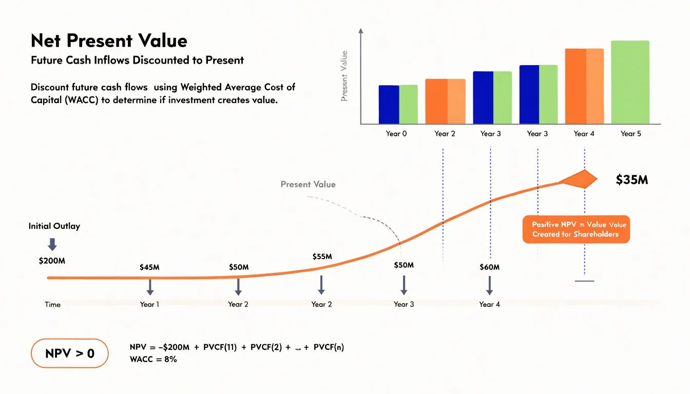
Net present value (NPV) is a fundamental concept in capital budgeting that incorporates the time value of money. The core principle is that a dollar received today is worth more than a dollar received in the future, because today’s dollar can be invested and earn a return. NPV applies this principle by discounting all expected future cash flows of a project back to the present using a discount rate, which reflects the opportunity cost of capital and the risk of those cash flows. The discount rate is typically the company’s weighted average cost of capital (WACC) or a rate that captures the riskiness of the project. By discounting each cash flow to its present value, NPV translates future dollars into today’s dollars, allowing for a direct comparison with the initial investment. A positive NPV means that the present value of the project’s cash inflows exceeds the present value of its outflows, including the initial cost. This indicates that the project is expected to generate more value than the required return, thereby creating value for shareholders. In essence, a positive NPV signals that the project earns a return greater than the cost of capital, increasing the firm’s value. Conversely, a negative NPV would destroy shareholder value. Therefore, the NPV rule states that a project should be accepted if its NPV is positive and rejected if negative. When choosing among mutually exclusive projects, the one with the highest NPV should be selected. The discount rate plays a critical role: a higher rate reduces the present value of future cash flows, making projects less attractive, while a lower rate increases present value. Thus, the choice of discount rate must accurately reflect the project’s risk and the firm’s opportunity cost of capital. NPV is widely preferred because it directly measures the change in shareholder wealth and accounts for the time value of money, risk, and all cash flows of the project.

Internal rate of return for comparing percentage yields

The internal rate of return is the discount rate at which a project’s net present value equals zero. In practical terms, it is the percentage yield a project is expected to generate over its life, given its stream of cash inflows and outflows. Calculating IRR involves solving for the rate r in the equation where the present value of all future cash flows, discounted at r, exactly offsets the initial investment. Because this equation cannot usually be solved analytically for multi-period projects, analysts rely on iterative numerical methods or spreadsheet functions to converge on the rate.

The appeal of IRR lies in its format. Expressing a project’s return as a single percentage makes it immediately comparable across proposals of different sizes, durations, and capital requirements. A manager can set IRR against the company’s cost of capital or a hurdle rate and see at a glance whether a project clears the bar. Ranking projects by IRR gives a quick sense of relative yield, and the measure is intuitive for communicating with non-financial stakeholders who find a percentage easier to interpret than a dollar-denominated NPV figure.

IRR does carry important limitations. The method assumes that interim cash flows are reinvested at the IRR itself, an assumption that can overstate returns when the IRR is high relative to realistic reinvestment opportunities. More significantly, IRR can behave unpredictably with non-conventional cash flows, meaning projects whose cash flow stream changes sign more than once, such as an initial outlay followed by inflows and then a later outflow for cleanup or refurbishment costs. In such cases the NPV profile can cross the zero line multiple times, producing more than one mathematically valid IRR. Deciding which rate to use then becomes ambiguous, and the measure may give no rate at all if the profile never crosses zero. When choosing among mutually exclusive projects, IRR can also mislead, because a smaller project with a high percentage return may add less absolute value than a larger project with a lower percentage return. Analysts therefore typically use IRR alongside NPV rather than in isolation, treating the percentage yield as a communication and screening tool while relying on NPV for the final value-based decision.

Payback Period

The payback period measures the length of time required for an investment to recover its initial cost from the cash inflows it generates. To calculate it, you accumulate the project’s net cash inflows year by year until the running total equals the original outlay. When inflows are uniform, the calculation is a simple division: initial investment divided by annual cash inflow. When inflows vary, you add full years of inflows until the cumulative figure approaches the initial cost, then estimate the fraction of the final year needed to close the gap. A project costing $100,000 that returns $25,000 each year, for example, has a payback period of four years.

The appeal of this measure lies in its directness. Managers can compute it quickly, explain it to non-specialists, and compare competing proposals on a single intuitive number. A shorter payback signals that capital is tied up for less time, which matters to firms with tight cash positions or limited access to external finance. The metric therefore serves as a rough liquidity screen, highlighting projects that return funds to the business quickly and reduce exposure to prolonged risk. Many organizations pair it with more rigorous techniques as an initial filter, discarding proposals whose payback stretches beyond an acceptable threshold before undertaking detailed analysis.

The limitations follow from the same narrow focus. Because the calculation stops the moment cumulative inflows match the initial outlay, every cash flow occurring after that cutoff is disregarded. Two projects with identical payback periods may differ enormously in later returns, and the payback rule cannot distinguish between them, so it may favor a modest early-recovery project over one with far greater long-term value. The measure also treats all cash flows as equal regardless of when they arrive, ignoring the time value of money. A dollar received in year one is weighted the same as a dollar received in year five, which overstates the attractiveness of projects with back-loaded returns. Discounted payback addresses this by discounting inflows before accumulation, though it still ignores everything beyond the break-even point. Understanding these trade-offs helps analysts use the payback period for what it does well, gauging recovery speed and liquidity, while relying on net present value or internal rate of return for judgments about overall profitability.

Profitability Index

The Profitability Index (PI) is a capital budgeting tool that measures the value created per unit of investment. It is calculated by dividing the present value of a project’s future cash flows by its initial investment. The formula is: PI = PV of future cash flows / Initial investment. This ratio provides a clear indicator of the relative profitability of a project, which is especially useful when a firm faces capital rationing—a situation where the available funds are insufficient to undertake all positive net present value (NPV) projects. Under capital rationing, the goal is to select the combination of projects that maximizes overall value given the limited capital. The PI helps in this ranking by showing how much value each project generates for every dollar invested. A PI greater than 1 indicates that the project’s present value of future cash flows exceeds the initial investment, meaning it has a positive NPV and should be considered acceptable. For example, a PI of 1.2 means that for every dollar invested, the project returns $1.20 in present value terms, creating $0.20 of value. A PI less than 1 signals that the project’s present value is less than the initial cost, resulting in a negative NPV, and it should generally be rejected. A PI exactly equal to 1 means the project breaks even in present value terms, with an NPV of zero. When ranking projects under capital rationing, the general rule is to prioritize projects with the highest PI, as they offer the greatest value per dollar of investment. However, this approach assumes that projects are independent and that the capital constraint is the only limiting factor. In practice, firms may also consider other factors such as project risk, strategic importance, and the size of the investment. The PI is particularly advantageous because it allows for a direct comparison of projects of different sizes, which NPV alone does not facilitate. For instance, a small project with a high PI may be preferred over a larger project with a lower PI when capital is limited, even if the larger project has a higher absolute NPV. Nonetheless, the PI should be used in conjunction with other techniques like NPV and IRR to ensure a comprehensive evaluation. By incorporating the PI into the capital budgeting process, managers can make more informed decisions about allocating scarce capital to projects that maximize firm value.

Accounting rate of return based on net income

The accounting rate of return (ARR) is a capital budgeting metric that evaluates a project by comparing its average annual net income to its initial or average investment. Unlike discounted cash flow methods, ARR draws directly from accrual accounting figures, specifically net income as reported on the income statement. This focus on net income rather than cash flows gives ARR a distinct appeal to managers whose performance is assessed on reported earnings. Because ARR aligns with the same accounting data used in financial statements, managers can readily see how a proposed project would affect the company’s reported profitability. This alignment can create an incentive to favor projects that boost net income in the short term, even if their cash flow characteristics are less favorable. However, this reliance on net income introduces several drawbacks. First, ARR ignores the time value of money. It treats a dollar of net income in year five the same as a dollar in year one, which can lead to biased comparisons between projects with different timing of income. Second, net income itself is subject to accounting conventions such as depreciation methods and revenue recognition policies, which can distort the true economic return. For example, a project with heavy early depreciation may show a low ARR even if its cash flows are strong. Additionally, ARR uses average annual net income, which smooths out year-to-year fluctuations but may obscure important patterns in cash flow timing. The metric also lacks a clear decision rule tied to shareholder value maximization; a project with an ARR above a target threshold may still destroy value if its cash flows are delayed or insufficient to cover the cost of capital. Despite these limitations, ARR remains popular in practice because it is simple to calculate from readily available accounting data and because it resonates with managers who are evaluated on accounting profits. Understanding both its appeal and its shortcomings helps analysts use ARR as a supplementary tool rather than a primary decision criterion.

Which method works best for small versus large projects

Choosing an appropriate capital budgeting method depends heavily on the scale, duration, and complexity of the project under consideration. For smaller, quicker projects, simpler techniques such as the payback period often provide sufficient guidance. A small equipment purchase, a minor facility upgrade, or a short-term marketing initiative typically involves modest capital outlay and a cash flow horizon measured in months rather than years. In these cases, the payback period offers a clear, intuitive answer to the central question: how soon will the investment return its cost? Managers can apply this method quickly without extensive forecasting infrastructure, making it well suited to high-volume, low-stakes decisions where the cost of detailed analysis would exceed any benefit gained from precision.

Larger, long-term investments present a different set of analytical demands. Projects such as plant construction, major technology platform implementations, or multi-year product development programs involve substantial capital commitments and cash flow patterns that unfold across many periods. These cash flows often include irregular timing, phased outlays, and terminal values that simple methods cannot capture adequately. Net present value and internal rate of return are better suited to this environment because they incorporate the time value of money and account for the full stream of cash flows over the project’s life. NPV expresses the expected value creation in absolute terms, giving decision-makers a direct measure of how much wealth the project is expected to add. IRR provides a comparable rate of return that can be weighed against the cost of capital and against competing proposals.

In practice, the choice also reflects organizational context. Smaller projects are often approved at lower management levels where speed matters and analytical resources are limited, while large investments typically undergo rigorous review by finance teams and executives who expect discounted cash flow analysis. Organizations commonly establish threshold policies, requiring payback analysis for projects below a certain dollar value and full NPV and IRR evaluation above it. This tiered approach balances analytical rigor against administrative cost, ensuring that the depth of analysis matches the significance of the decision at hand.

How do you handle conflicting results between NPV and IRR

Conflicts between NPV and IRR arise because the two metrics answer different questions and rely on different assumptions. NPV measures the absolute increase in firm value from a project, discounting all cash flows at the required rate of return. IRR, by contrast, finds the discount rate that makes a project’s NPV zero, effectively expressing return as a percentage. When comparing mutually exclusive projects, these differences can lead to divergent rankings.

Scale is a common source of conflict. A small project may have a high IRR but a modest NPV, while a larger project may have a lower IRR but a greater NPV. For example, Project A requires $10,000 and returns 50%, generating an NPV of $2,000; Project B requires $100,000 and returns 30%, generating an NPV of $10,000. IRR favors A, but B adds more value in absolute terms. If the goal is to maximize shareholder wealth, B is preferable despite its lower percentage return.

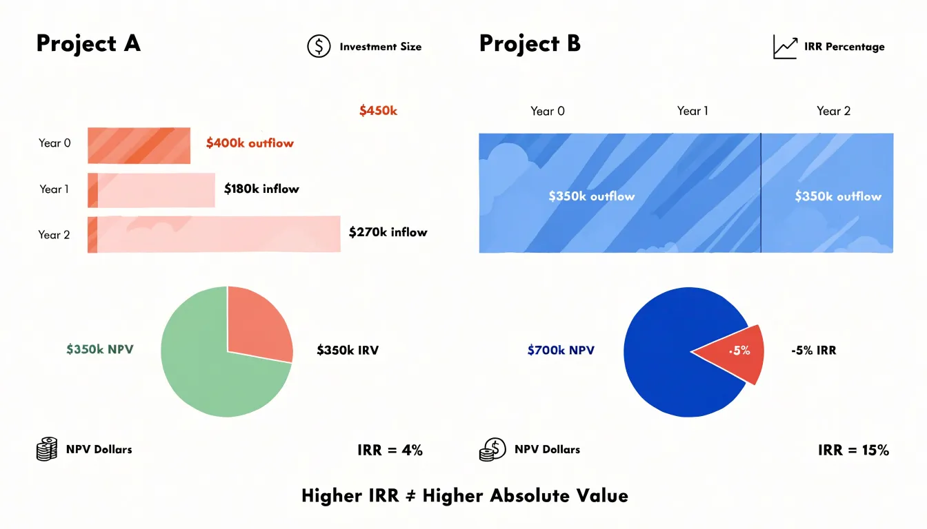
Timing of cash flows also matters. Projects with early cash inflows tend to have higher IRRs because those flows are less heavily discounted. A project with later, larger cash flows may have a lower IRR but a higher NPV when discounted at the firm’s cost of capital. The IRR’s implicit reinvestment rate assumption—that interim cash flows are reinvested at the IRR itself—can be unrealistic, especially for projects with very high IRRs. NPV assumes reinvestment at the cost of capital, which is more conservative and generally more realistic.

The reinvestment rate assumption is a key theoretical difference. IRR assumes cash flows are reinvested at the IRR, which may not reflect actual opportunities. NPV assumes reinvestment at the required rate of return, a more defensible assumption for most firms. This can cause IRR to overstate the true return of projects with high early cash flows.

Given these issues, NPV should generally take precedence for value maximization. NPV directly measures the expected change in firm value and aligns with the goal of shareholder wealth maximization. It avoids the pitfalls of percentage-based rankings and unrealistic reinvestment assumptions. IRR remains useful as a supplementary measure, offering insight into a project’s safety margin and return profile, but when the two conflict, the NPV rule provides a more reliable guide for capital allocation decisions.

Real-world traps that mess up long-term cash flow estimates

Long-term cash flow estimates sit at the heart of any capital budgeting decision, and they are also where the analysis most often goes wrong. A handful of recurring pitfalls trip up even experienced analysts, and each one can quietly distort a project’s apparent value.

Overoptimistic revenue forecasts are the most common trap. Projections built on best-case scenarios, rosy market-share assumptions, or a single enthusiastic sales forecast tend to overstate early cash inflows. Analysts often anchor on the sponsor’s numbers, which carry an incentive to inflate. A disciplined approach builds revenue from verifiable demand drivers and stress-tests the top line against historical analogues.

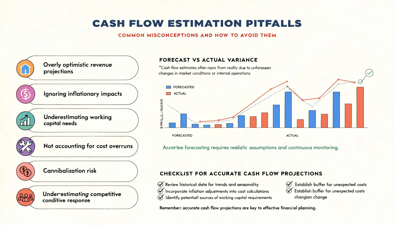
Ignoring inflation is a subtler error. Forecasts that use today’s prices while applying a nominal discount rate understate future cash flows, while mixing real and nominal figures produces inconsistent results. Likewise, working capital is often treated as an afterthought. Growing operations tie up cash in receivables and inventory, and a project that looks attractive on operating cash flow alone can strain liquidity once those needs are included. Every incremental dollar of sales usually requires incremental working capital, and that cash must be recovered in the terminal year.

Cost underestimation follows a well-documented pattern. Capital projects routinely run over budget and take longer than planned, and ongoing operating costs are frequently understated. Contingency allowances and a realistic ramp-up period belong in any credible model.

Finally, analysts often evaluate a project in isolation. Cannibalization is a real cost: a new product line may steal sales from existing offerings, so incremental cash flow must be measured net of lost revenue elsewhere. Competitive responses matter too. Rivals may cut prices, launch substitutes, or expand capacity, eroding the margins the forecast assumed. Building these dynamics into the model, rather than assuming a static competitive landscape, produces far more reliable estimates.

Each of these traps shares a root cause: the tendency to treat projections as confirmations of a decision already made. Rigorous cash flow estimation requires humility, skepticism, and a willingness to model the downside as carefully as the upside.

Frequently Asked Questions

Why is capital budgeting important for major business investments?

Major business investments lock up substantial resources for years and are often largely irreversible, so a single poor decision can strain liquidity, raise borrowing costs, and depress earnings. Structured capital budgeting imposes discipline by forcing managers to quantify expected cash flows, assess risk, and justify the commitment before funds are spent.

What does a positive NPV mean?

A positive NPV means the present value of a project’s cash inflows exceeds the present value of its outflows, including the initial cost, so it is expected to earn more than the required return and create shareholder value. The NPV rule is to accept positive-NPV projects and reject negative-NPV projects, and when choosing among mutually exclusive projects, select the one with the highest NPV.

What are the main drawbacks of using IRR?

IRR assumes interim cash flows are reinvested at the IRR itself, which can overstate returns, and it can behave unpredictably with non-conventional cash flows by producing more than one valid IRR or no rate at all. When choosing among mutually exclusive projects, IRR can also mislead because a smaller project with a high percentage return may add less absolute value than a larger project with a lower percentage return. Analysts therefore typically use IRR alongside NPV rather than in isolation.

How do you calculate the payback period?

The payback period is the time required for a project’s cash inflows to recover its initial cost. If inflows are uniform, divide the initial investment by the annual cash inflow; if they vary, accumulate inflows year by year and estimate the fraction of the final year needed to close the gap.

What does a profitability index greater than 1 mean?

A PI greater than 1 means the present value of future cash flows exceeds the initial investment, indicating a positive NPV, and the project should be considered acceptable. A PI less than 1 signals a negative NPV and should generally be rejected, while a PI exactly equal to 1 means the project breaks even in present value terms.

How do you handle conflicting NPV and IRR results?

NPV should generally take precedence for value maximization because it directly measures the expected change in firm value. IRR remains useful as a supplementary measure, but when the two conflict, the NPV rule provides a more reliable guide for capital allocation decisions.