How to Calculate Loan Payments by Hand or in Excel

Loan payments are calculated using the formula M = P × [i(1 + i)^n] ÷ [(1 + i)^n − 1], where P is principal, i is the monthly interest rate (annual rate divided by 12), and n is the total number of monthly payments. In Excel, the equivalent is =PMT(rate, nper, pv), with rate and nper in matching monthly units.

Understanding the Core Variables Behind Every Loan

Every loan payment calculation rests on three inputs, and understanding what each one represents makes the math far less mysterious. The first is the principal, which is the original amount borrowed. If you take out a $20,000 loan, that $20,000 is the principal. It forms the base of the calculation because interest is charged against the outstanding balance, so a larger principal means more interest accrues and a higher monthly payment. As you make payments over time, the principal balance shrinks, which is why the interest portion of each payment gradually declines.

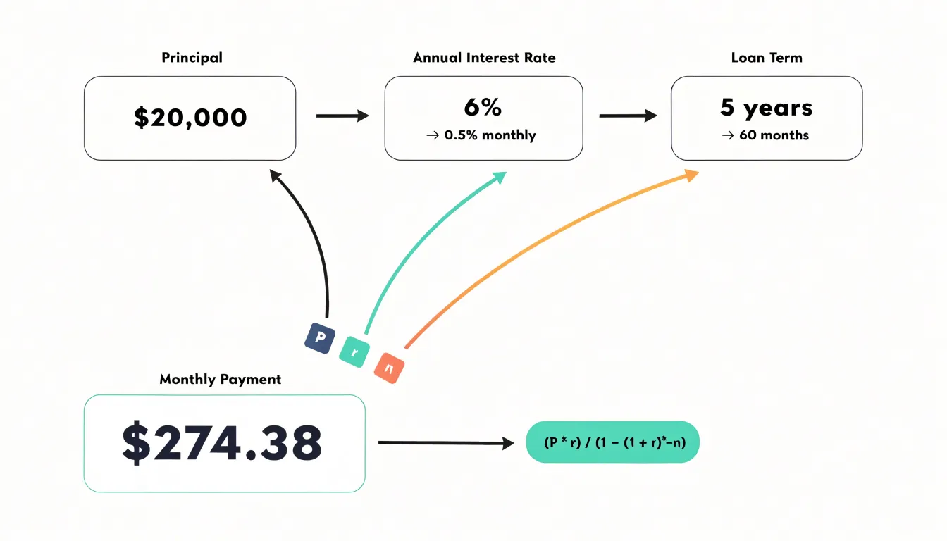
The second variable is the interest rate, typically expressed as an annual percentage rate (APR). Lenders quote rates on an annual basis, but loan payments are usually made monthly, so the annual rate must be divided by 12 to get the monthly rate. A 6% annual rate becomes 0.5% per month. Because interest is calculated on the remaining balance each period, even a small difference in rate can produce a noticeable change in the payment. A rate of 6% versus 7% on the same principal and term can shift the monthly figure by tens of dollars and add thousands over the life of the loan.

The third variable is the loan term, which is the number of months over which the loan is scheduled to be repaid. A 30-year mortgage has 360 monthly periods, while a five-year auto loan has 60. The term interacts directly with the rate: stretching repayment over more periods lowers each individual payment but increases the total interest paid, because the balance stays outstanding longer. Shortening the term raises the monthly payment while reducing total interest.

These three inputs—principal, monthly interest rate, and number of periods—feed into the standard amortization formula. Once you identify each value, you can plug them into the formula or a spreadsheet function and arrive at an accurate payment figure. Recognizing how each variable moves the result also lets you compare loan offers knowledgeably and see the trade-offs between payment size and total cost.

Why Should You Learn the Math Before Using a Spreadsheet?

Learning the math behind a loan payment before relying on a spreadsheet gives you a foundation that makes every later calculation easier to trust. A spreadsheet is a fast tool, and speed is exactly where small mistakes hide. A misplaced parenthesis, a rate entered as a percentage instead of a decimal, or a term expressed in years where months are expected can all produce a payment figure that looks plausible on screen while being badly wrong. When you understand how the payment is built from principal, interest rate, and number of periods, you can spot those errors immediately because you know roughly what the answer should look like.

That rough expectation is the real payoff. Someone who has worked the formula by hand knows that a five-year loan at a given rate should produce a payment in a particular range. If a spreadsheet returns a number far outside that range, the discrepancy stands out as a warning rather than slipping past unnoticed. This habit of checking results against an independent estimate is one of the simplest forms of error detection available, and it costs only a few minutes.

Understanding the underlying math also lets you verify a lender’s figures with confidence. Loan documents, payoff quotes, and amortization schedules are prepared by other people, and occasionally they contain mistakes or use conventions you did not expect. A borrower who can reconstruct the payment from the basic inputs is in a position to ask informed questions and catch discrepancies before signing. Without that knowledge, the same borrower has little choice but to accept whatever number appears on the page.

The deeper benefit is the ability to reason about trade-offs. Once the formula is familiar, you can see how each input drives the result: how a longer term lowers the monthly payment while raising total interest, how a small change in rate shifts the balance over time, and how extra payments shorten the schedule. These insights support real decisions about affordability, refinancing, and repayment strategy. The spreadsheet remains useful for speed and for modeling many scenarios, yet it becomes a tool you direct rather than a black box you consult. That shift from trusting output to understanding it is what turns a borrower into an informed one.

The Standard Payment Formula Broken Down Simply

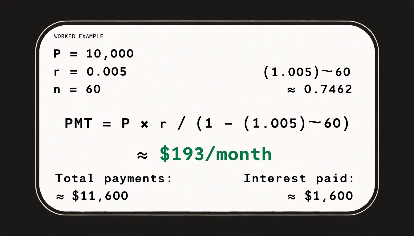
The standard loan payment formula, often labeled PMT in financial contexts, gives you the fixed amount you pay each period on an amortizing loan. In plain English, the formula is: Payment equals the principal times the periodic rate, divided by one minus the quantity one plus the periodic rate raised to the negative number of periods. Written compactly, PMT = P × r / (1 − (1 + r)^−n). Each piece of that expression has a straightforward meaning, and once you understand the parts, the whole calculation becomes much less intimidating.

Start with P, the principal. This is the original amount you borrow, before any interest is added. Next is r, the periodic interest rate. Lenders usually quote an annual percentage rate, so you divide that annual rate by the number of payment periods in a year. A loan with a 6 percent annual rate paid monthly uses a periodic rate of 0.06 divided by 12, or 0.005. The third component, n, is the total number of payment periods. A five-year loan with monthly payments has n equal to 60 periods. These three values are the only inputs you need.

The denominator, 1 − (1 + r)^−n, deserves a moment of attention because it is where most people get lost. It represents a discounting factor that converts a stream of equal future payments into a single present value. When r is small and n is large, this factor approaches a number close to 1 minus a tiny fraction, which makes the division behave predictably. You do not need to interpret it deeply to use it; treat it as a conversion step that adjusts the interest portion of your payment across the life of the loan.

A quick example ties everything together. Suppose you borrow 10,000 dollars at 6 percent annual interest for five years, paid monthly. Here P is 10,000, r is 0.005, and n is 60. Compute (1.005)^−60, subtract that result from 1, then divide 10,000 times 0.005 by the result. The payment comes out to roughly 193 dollars per month. From there, multiplying by 60 gives total payments of about 11,600 dollars, so the interest cost is around 1,600 dollars. That single calculation reveals the full cost of borrowing.

Step-by-step Guide

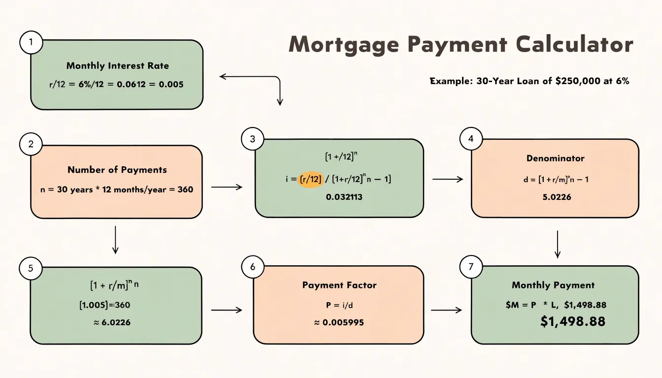
The formula for a fixed-rate loan payment is M = P × [i(1 + i)^n] ÷ [(1 + i)^n − 1], where M is the monthly payment, P is the principal, i is the monthly interest rate, and n is the total number of payments. Working through it by hand rewards careful attention to order of operations, so it helps to break the calculation into small, numbered stages and write down each result before moving on.

Begin by converting the annual interest rate to a monthly rate. For a 6 percent annual rate, divide 0.06 by 12 to get i = 0.005. Next, find n by multiplying the loan term in years by 12; a 30-year loan gives n = 360. With those two figures in hand, compute the compound factor (1 + i)^n. Add 1 to the monthly rate to get 1.005, then raise it to the 360th power. A scientific calculator handles this in one keystroke, yielding approximately 6.0226. Keep four decimal places for accuracy.

Now build the numerator by multiplying that result by i: 6.0226 × 0.005 = 0.030113. Build the denominator by subtracting 1 from the compound factor: 6.0226 − 1 = 5.0226. Divide the numerator by the denominator to obtain the payment factor: 0.030113 ÷ 5.0226 ≈ 0.005995. This figure represents the monthly payment per dollar borrowed.

Apply the factor to the principal. On a $250,000 loan, multiply 250,000 × 0.005995, which gives a monthly payment of about $1,498.88. Round only at the final step, since rounding intermediate figures can shift the answer by several dollars over a long term.

As a sanity check, compare the total of all payments to the amount borrowed. Here, 360 payments of $1,498.88 come to roughly $539,597, so interest costs about $289,597 across the life of the loan. Running the numbers a second time, or verifying the payment factor with an online calculator, catches arithmetic slips before they propagate. Practicing the sequence on a few different loan amounts builds familiarity with how each input moves the final figure.

Excel PMT Function

Excel’s PMT function computes the constant payment required to pay off a loan over a fixed number of periods at a fixed interest rate, and it returns the result instantly once you supply the inputs correctly. The full syntax is =PMT(rate, nper, pv, [fv], [type]). Each argument occupies a specific position, and the order matters because Excel does not accept named arguments in the formula bar the way some programming languages do. The rate argument is the interest rate per period, so a 6 percent annual loan paid monthly requires 0.06 divided by 12, or 0.005. The nper argument is the total number of payment periods, which for a five-year monthly loan is 60. The pv argument is the present value, meaning the loan amount you are borrowing, entered as a positive number. The optional fv argument represents a future value or balloon balance remaining after the last payment, and it defaults to zero for a fully amortizing loan. The optional type argument specifies whether payments occur at the end of each period (0 or omitted) or the beginning (1).

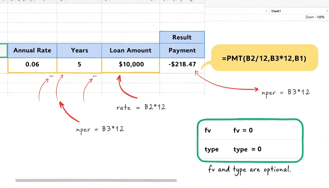
Sign conventions trip up many first-time users. Excel treats cash flows directionally: money you receive and money you pay must carry opposite signs. If you enter the loan amount as a positive 20000 in the pv position, the PMT function returns a negative number because the payments represent money leaving your pocket. Wrapping the formula in a minus sign, as in =-PMT(0.005, 60, 20000), produces a positive payment figure that reads more naturally on a budget sheet. Mixing signs inconsistently, such as entering a negative loan amount and expecting a positive result, produces confusing output and is the most common source of errors.

A second pitfall involves mismatching the rate and period units. Dividing an annual rate by 12 while entering the term in years, rather than months, yields a wildly incorrect payment. Always express rate and nper in the same time unit. Rounding the rate too aggressively before entry can also shift results noticeably on large loans. Finally, remember that PMT returns only principal and interest; property taxes, insurance, and fees must be added separately to arrive at a true monthly housing cost. With the arguments in the right order and signs handled deliberately, the function delivers an accurate payment figure in a single cell.

How to Build a Complete Amortization Schedule in Excel

Building a complete amortization schedule in Excel turns a single monthly payment figure into a full picture of how a loan behaves over its entire life. Start by setting up a small input area at the top of the sheet with the loan amount, annual interest rate, loan term in years, and payments per year. From these inputs, calculate the periodic interest rate by dividing the annual rate by the number of payments per year, and calculate the total number of payments by multiplying the term by the payments per year. The payment itself comes from the PMT function, referencing these cells so the whole sheet updates whenever an input changes.

Below the inputs, create a table with columns for payment number, beginning balance, payment amount, interest portion, principal portion, and ending balance. In the first row, the beginning balance equals the original loan amount, the payment references the PMT result, and the interest portion is the beginning balance multiplied by the periodic rate. The principal portion is the payment minus the interest, and the ending balance is the beginning balance minus the principal. For the second row, the beginning balance simply references the ending balance of the first row, and every other formula can be copied down.

Drag the formulas down for the total number of payments. As you scroll through the table, you will see the interest portion shrink and the principal portion grow with each row, illustrating how early payments go mostly toward interest while later payments chip away at the balance. The final ending balance should land at or very near zero, which serves as a check that the schedule is built correctly.

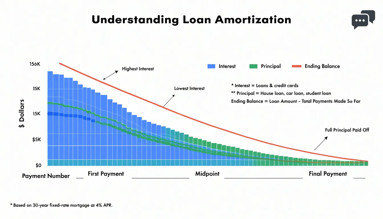
A few refinements make the schedule more useful. Use absolute references for the rate and payment cells so copied formulas stay accurate. Format the currency columns consistently, and apply conditional formatting to highlight the point where cumulative principal exceeds cumulative interest. You can also add a summary row using SUM to total the interest and principal paid over the life of the loan, giving you a clear figure for the true cost of borrowing.

How Do Extra Principal Payments Change Your Repayment Timeline?

Extra principal payments change the structure of a loan in a way that compounds quietly over time. On an amortized loan, each monthly payment splits into two parts: interest, calculated on the remaining balance, and principal, which reduces that balance. When you add extra money toward principal, the balance drops faster than the original schedule anticipates. Because the following month’s interest is calculated on a smaller balance, more of the regular payment flows toward principal, which reduces the balance further still. This feedback loop accelerates as the loan matures, meaning modest additional amounts made early in the loan produce outsized savings in both interest and time.

The interest savings come from the fact that every dollar of principal retired early never gets charged interest for the remaining months of the term. A borrower who adds even a small fixed amount each month can shave years off a thirty-year mortgage and save tens of thousands in interest, depending on the rate and balance. The timeline effect follows the same logic: reducing the balance shortens the number of payments needed to reach zero, and the loan is retired at the point where the balance hits zero rather than at the originally scheduled maturity date.

Modeling this in Excel requires a row-by-row amortization schedule. Set up columns for payment number, beginning balance, the regular payment (using PMT), the interest portion (beginning balance times the monthly rate), the principal portion (payment minus interest), any extra principal, and the ending balance. The ending balance formula subtracts both the regular principal and the extra principal from the beginning balance, and the next row’s beginning balance references that ending balance. Once the schedule is built, add an extra principal column with a fixed value or a percentage of the payment, then let the recalculated ending balances flow down the rows. The row where the balance first crosses zero marks the new payoff date, and summing the interest column gives the total interest paid. Comparing that sum against the original schedule’s total interest quantifies the savings, while counting the rows to the zero balance shows the term reduction in months. Data tables can extend this analysis by testing several extra-payment amounts side by side.

Troubleshooting Common Calculation Mistakes and Formula Errors

When a loan payment calculation produces a result that looks wrong, the cause is usually one of a handful of recurring mistakes. One of the most frequent is entering an annual interest rate directly into a monthly payment formula. The standard amortization formula expects the periodic rate, meaning the annual rate divided by the number of payment periods per year. If a 6 percent annual rate is typed in as 6 rather than 0.005, the calculated payment will be wildly inflated. The fix is to confirm the rate basis before running the numbers and to keep the conversion consistent throughout the spreadsheet. The same logic applies to the number of periods: a five-year loan paid monthly requires 60 periods, so multiplying years by the payment frequency catches mismatches quickly.

Parentheses and operator order create another common source of errors, especially in Excel. Formulas like =PMT(rate, nper, pv) depend on the arguments appearing in the correct sequence and on negative signs being used for cash outflows. A misplaced parenthesis can silently change a subtraction into a multiplication, or cause the exponent in a denominator to apply to the wrong term. When a result seems off by a factor or comes out negative when it should be positive, break the formula into its component parts in separate cells and check each piece. Laying out the periodic rate, the period count, and the present value individually makes it easy to spot where the structure broke down.

Fees and other charges are often left out of the calculation entirely, which makes the quoted payment look better than the loan actually is. Origination fees, insurance, and closing costs may be financed into the principal or charged separately, and each treatment changes the payment. Reread the loan agreement to see which costs are rolled into the amount borrowed and which are paid upfront. If a lender quotes an APR, that figure already incorporates certain fees, and comparing a hand-calculated payment against the quoted APR is a good cross-check.

Finally, rounding at intermediate steps can introduce small but persistent discrepancies. Carry full precision until the final result, then round only the displayed payment, and verify totals against the lender’s amortization schedule.

Frequently Asked Questions

What three inputs do I need to calculate a loan payment?

You need the principal, the periodic interest rate, and the number of payment periods. The annual rate is divided by 12 for monthly payments, and the loan term in years is multiplied by 12 to get the number of monthly periods.

What is the standard formula for calculating a loan payment by hand?

The standard formula is PMT = P × r / (1 − (1 + r)^−n), where P is principal, r is the periodic interest rate, and n is the total number of payment periods. Another version in the article is M = P × [i(1 + i)^n] ÷ [(1 + i)^n − 1].

How do I use Excel’s PMT function to calculate a loan payment?

Use =PMT(rate, nper, pv, [fv], [type]), where rate is the interest rate per period, nper is the total number of payment periods, and pv is the loan amount entered as a positive number. If pv is positive, PMT returns a negative payment because cash flows have opposite signs, so wrapping the formula in a minus sign produces a positive payment figure.

How do I build a complete amortization schedule in Excel?

Set up inputs for the loan amount, annual interest rate, loan term, and payments per year, then calculate the periodic rate, total number of payments, and payment with PMT. Create columns for payment number, beginning balance, payment amount, interest portion, principal portion, and ending balance, and copy the formulas down for the total number of payments.

How do extra principal payments change a loan’s repayment timeline?

Extra principal payments lower the balance faster, so the following month’s interest is calculated on a smaller balance and more of the regular payment goes toward principal. This can shorten the number of payments needed to reach zero and reduce total interest paid.

What common mistakes can make a loan payment calculation wrong?

Common mistakes include entering an annual interest rate directly into a monthly payment formula, mismatching the rate and period units, misplacing parentheses, leaving out fees, and rounding at intermediate steps. To catch errors, keep rate and period units consistent, carry full precision until the final result, and verify totals against the lender’s amortization schedule.